How To: Analyze Wi-Fi Data Captures with Jupyter Notebook

When it comes to sniffing Wi-Fi, Wireshark is cross-platform and capable of capturing vast amounts of data. Making sense of that data is another task entirely. That's where Jupyter Notebook comes in. It can help analyze Wi-Fi packets and determine which networks a particular phone has connected to before, giving us insight into the identity of the owner.

Overall, data can be confusing, especially when there's a lot of it, which is both a blessing and a curse. It makes it more likely to include important patterns, but also more likely to obscure them. Looking for meaningful patterns in raw data can be like finding a needle in a haystack, but free tools for big data analysis, such as Jupyter Notebook, make things easier.

Wireshark for Wi-Fi Data

Wireshark is an incredible tool for gathering Wi-Fi data, and it can quickly fill up a screen with information. That data can tell you a lot, depending on what you're looking for, but it's often saying too much to be able to recognize patterns easily. Wireshark does come with built-in ways to analyze data, but sharing the results can be difficult, and the tools built into Wireshark may not be able to tell you what you need.

The kind of data you can get from a Wireshark capture includes the MAC addresses of every device transmitting or receiving nearby, information about which clients are connected to which networks currently, and even information about networks nearby clients have connected to in the past.

• More Info: Spy on Traffic from a Smartphone with Wireshark

All of that can be very valuable to a hacker interested in tracking the location or learning information about a subject. Finding Wi-Fi networks a device has connected to before will also allow an attacker to create fake versions of trusted networks that the victim's device will connect to automatically.

Jupyter Notebook for Data Analysis

Once we've gathered information in Wireshark, we can export it as a CSV file and import it into Jupyter Notebook. The benefit of doing so is that we can quickly slice through the data generated by Wireshark using Python's Pandas library. That library can work with CSV files as data frames, which can easily plot graphs and charts of data to show relationships.

One of the nice things about working with Jupyter Notebook is how easy it is to dig through information for insights. A significant difference between data and intelligence is processing the data into insights, which is what working with data in Jupyter allows us to do.

In our example, we'll be using Jupyter Notebook to examine a Wireshark capture on a public train. In the capture, we are recording the devices of passengers responding to the Arduino "Beacon Spammer" sketch, which creates 40 fake Wi-Fi APs with the names of popular open networks. Any device which has joined a hotspot with the same name as one of the fake ones will attempt to connect. We can record and graph these responses in Jupyter Notebook to learn which fake networks cause the most phones to react and which of the phony network names each phone has connected to in the past.

• More Info Use an ESP8266 Beacon Spammer to Track Smartphone Users

What You'll Need

To follow along, you'll need a computer with Wireshark. It helps to have a card that can be put into monitor mode, but you can also use data from the capture on GitHub to follow along if you can't generate your own. You can download the sample CSV dataset by cloning the repo, changing into its directory, and listing its contents.

• Don't Miss: The Best Wireless Network Adapter for Wi-Fi Hacking

~# git clone https://github.com/skickar/Research.git

Cloning into 'Research'...
remote: Enumerating objects: 21, done.
remote: Counting objects: 100% (21/21), done.
remote: Compressing objects: 100% (21/21), done.
remote: Total 107 (delta 9), reused 0 (delta 0), pack-reused 86
Receiving objects: 100% (107/107), 1.18 MiB | 4.91 MiB/s, done.
Resolving deltas: 100% (47/47), done.

~# cd Research
~/Research# ls

commands.json     jsonpayload.json                             sash.json
dataCleaner.py    MetroWilshireVermonttoHollywoodHighland.csv  SocalDecloaker.ino
fades.py          NullByteSpecial.ipynb                        twitter0.json
FindWiFiDistance  README.md                                    twitter1.json
json.json         RedLineResearch.ipynb

You'll also need Python3 to run Jupyter, so make sure your system has it before continuing.

To retry the experiment and capture your own data, you need to use the Beacon Spammer sketch on an ESP8266-based device, set to stay on the channel of your choice. You should add common network names that require no password from your area, up to 1,000. When you flash the sketch and plug in the ESP8266, you should see the fake networks appear.

Then, you'll need to record in Wireshark only on the channel you specified. Record all of the traffic while the Beacon Spammer is running to watch for devices trying to connect. The resulting data should work fine for us to analyze.

Step 1: Export a Wireshark Capture as a CSV File

First, we'll take a PCAP file in Wireshark and turn it into a CSV file to use in Jupyter Notebook. To do so, open your capture in Wireshark, and add any data you need from packets to the columns by right-clicking on the field you want to add and select "Apply as Column."

Next, add any display filters you want to eliminate unwanted packets. Here, I'm saying I only want packets with a destination address matching the partial MAC address "6c:3f:23." This capture filter also uses the [0:3] to specify I want to look from the beginning to the third octet of the MAC address.

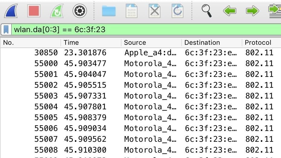
Once the capture filter is up, only packets sent to the Beacon Spammer are seen. Each time we start the Beacon Spammer, it picks a MAC address and then changes the last half of the MAC for each fake network it creates. That makes it easy to select all the packets sent to our fake networks by telling Wireshark only to include packets sent to addresses that have the same partial MAC address.

Finally, it's time to export our selected packets. Under "File," click on "Export Packet Dissections" and select "As CSV" to export in the right format.

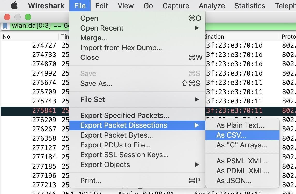
Here, you can name the file and specify if you want the displayed packets to be exported or all packets in the capture.

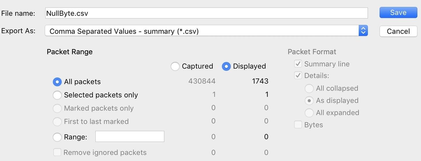
Once that's done, a CSV file containing the data should be saved to your computer, ready to import into Jupyter Notebook.

Step 2: Install Jupyter & Open a New Notebook

Jupyter is a data analysis program that's written in Python, which makes it simple to install on any computer with Python3 installed. You can do so by running the following command in a new terminal window.

~# pip3 install jupyter

Requirement already satisfied: jupyter in /usr/local/lib/python3.7/dist-packages (1.0.0)
Requirement already satisfied: notebook in /usr/local/lib/python3.7/dist-packages (from jupyter) (6.0.2)
Requirement already satisfied: jupyter-console in /usr/local/lib/python3.7/dist-packages (from jupyter) (6.0.0)
Requirement already satisfied: nbconvert in /usr/local/lib/python3.7/dist-packages (from jupyter) (5.6.1)
Requirement already satisfied: ipywidgets in /usr/local/lib/python3.7/dist-packages (from jupyter) (7.5.1)
Requirement already satisfied: ipykernel in /usr/local/lib/python3.7/dist-packages (from jupyter) (5.1.3)
Requirement already satisfied: qtconsole in /usr/local/lib/python3.7/dist-packages (from jupyter) (4.6.0)
Requirement already satisfied: jupyter-client>=5.3.4 in /usr/local/lib/python3.7/dist-packages (from notebook->jupyter) (5.3.4)
Requirement already satisfied: Send2Trash in /usr/local/lib/python3.7/dist-packages (from notebook->jupyter) (1.5.0)
Requirement already satisfied: prometheus-client in /usr/local/lib/python3.7/dist-packages (from notebook->jupyter) (0.7.1)
Requirement already satisfied: pyzmq>=17 in /usr/local/lib/python3.7/dist-packages (from notebook->jupyter) (18.1.1)
Requirement already satisfied: terminado>=0.8.1 in /usr/local/lib/python3.7/dist-packages (from notebook->jupyter) (0.8.3)
Requirement already satisfied: jupyter-core>=4.6.0 in /usr/local/lib/python3.7/dist-packages (from notebook->jupyter) (4.6.1)
Requirement already satisfied: nbformat in /usr/lib/python3/dist-packages (from notebook->jupyter) (4.4.0)
Requirement already satisfied: traitlets>=4.2.1 in /usr/lib/python3/dist-packages (from notebook->jupyter) (4.3.2)
Requirement already satisfied: jinja2 in /usr/lib/python3/dist-packages (from notebook->jupyter) (2.10)
Requirement already satisfied: tornado>=5.0 in /usr/lib/python3/dist-packages (from notebook->jupyter) (5.1.1)
Requirement already satisfied: ipython-genutils in /usr/lib/python3/dist-packages (from notebook->jupyter) (0.2.0)
Requirement already satisfied: prompt-toolkit<2.1.0,>=2.0.0 in /usr/local/lib/python3.7/dist-packages (from jupyter-console->jupyter) (2.0.10)
Requirement already satisfied: pygments in /usr/lib/python3/dist-packages (from jupyter-console->jupyter) (2.3.1)
Requirement already satisfied: ipython in /usr/local/lib/python3.7/dist-packages (from jupyter-console->jupyter) (7.10.2)
Requirement already satisfied: testpath in /usr/local/lib/python3.7/dist-packages (from nbconvert->jupyter) (0.4.4)
Requirement already satisfied: mistune<2,>=0.8.1 in /usr/local/lib/python3.7/dist-packages (from nbconvert->jupyter) (0.8.4)
Requirement already satisfied: pandocfilters>=1.4.1 in /usr/local/lib/python3.7/dist-packages (from nbconvert->jupyter) (1.4.2)
Requirement already satisfied: entrypoints>=0.2.2 in /usr/lib/python3/dist-packages (from nbconvert->jupyter) (0.3)
Requirement already satisfied: defusedxml in /usr/local/lib/python3.7/dist-packages (from nbconvert->jupyter) (0.6.0)
Requirement already satisfied: bleach in /usr/local/lib/python3.7/dist-packages (from nbconvert->jupyter) (3.1.0)
Requirement already satisfied: widgetsnbextension~=3.5.0 in /usr/local/lib/python3.7/dist-packages (from ipywidgets->jupyter) (3.5.1)
Requirement already satisfied: python-dateutil>=2.1 in /usr/lib/python3/dist-packages (from jupyter-client>=5.3.4->notebook->jupyter) (2.7.3)
Requirement already satisfied: ptyprocess; os_name != "nt" in /usr/local/lib/python3.7/dist-packages (from terminado>=0.8.1->notebook->jupyter) (0.6.0)
Requirement already satisfied: six>=1.9.0 in /usr/lib/python3/dist-packages (from prompt-toolkit<2.1.0,>=2.0.0->jupyter-console->jupyter) (1.12.0)
Requirement already satisfied: wcwidth in /usr/local/lib/python3.7/dist-packages (from prompt-toolkit<2.1.0,>=2.0.0->jupyter-console->jupyter) (0.1.7)
Requirement already satisfied: pickleshare in /usr/local/lib/python3.7/dist-packages (from ipython->jupyter-console->jupyter) (0.7.5)
Requirement already satisfied: backcall in /usr/local/lib/python3.7/dist-packages (from ipython->jupyter-console->jupyter) (0.1.0)
Requirement already satisfied: decorator in /usr/lib/python3/dist-packages (from ipython->jupyter-console->jupyter) (4.3.0)
Requirement already satisfied: pexpect; sys_platform != "win32" in /usr/local/lib/python3.7/dist-packages (from ipython->jupyter-console->jupyter) (4.7.0)
Requirement already satisfied: setuptools>=18.5 in /usr/lib/python3/dist-packages (from ipython->jupyter-console->jupyter) (40.8.0)
Requirement already satisfied: jedi>=0.10 in /usr/local/lib/python3.7/dist-packages (from ipython->jupyter-console->jupyter) (0.15.2)
Requirement already satisfied: webencodings in /usr/lib/python3/dist-packages (from bleach->nbconvert->jupyter) (0.5.1)
Requirement already satisfied: parso>=0.5.2 in /usr/local/lib/python3.7/dist-packages (from jedi>=0.10->ipython->jupyter-console->jupyter) (0.5.2)

Once Jupyter is installed, we can run it to create a web interface and open it automatically. To do so, type the following. If you run as root, you'll get a prompt telling you that it's not recommended, and you can choose to continue or switch accounts.

~# jupyter notebook

[I 00:26:51.488 NotebookApp] JupyterLab extension loaded from /Library/Frameworks/Python.framework/Versions/3.6/lib/python3.6/site-packages/jupyterlab
[I 00:26:51.488 NotebookApp] JupyterLab application directory is /Library/Frameworks/Python.framework/Versions/3.6/share/jupyter/lab
[I 00:26:51.490 NotebookApp] Serving notebooks from local directory: /Users/skickar
[I 00:26:51.491 NotebookApp] The Jupyter Notebook is running at:
[I 00:26:51.491 NotebookApp] http://localhost:8888/?token=4de1f5eba5b656d903d08298a831a11ba97a581e3e575cda
[I 00:26:51.491 NotebookApp] Use Control-C to stop this server and shut down all kernels (twice to skip confirmation).
[C 00:26:51.496 NotebookApp]

    To access the notebook, open this file in a browser:
        file:///Users/skickar/Library/Jupyter/runtime/nbserver-54785-open.html
    Or copy and paste one of these URLs:
        http://localhost:8888/?token=4de1f5eba5b656d903d08298a831a11ba97a581e3e575cda

A web browser should open, allowing you to select previous projects or open a new one.

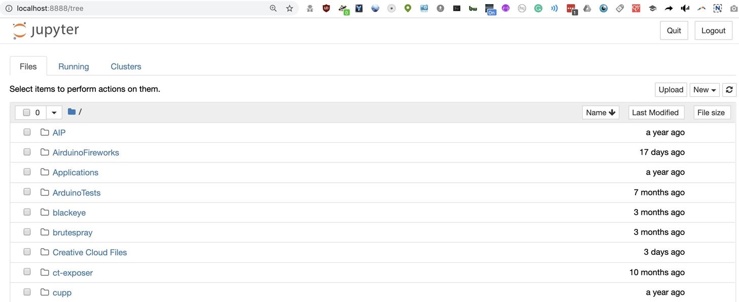
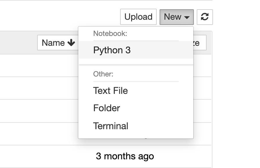
Click "New" and then "Python 3" to open a new notebook.

Step 3: Import Data in Jupyter

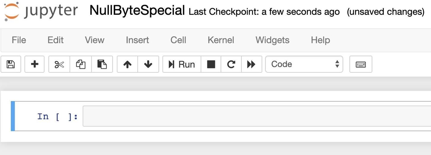
Let's take a look at the layout. At the top, we'll see options to save, insert an input, and run commands. We'll also see the "In" prompt, waiting for us to add some Python 3.

Now, we'll need to import our Wireshark CSV file into a Pandas data frame. The Pandas and Matplotlib libraries will help us easily work with and manipulate captured data.

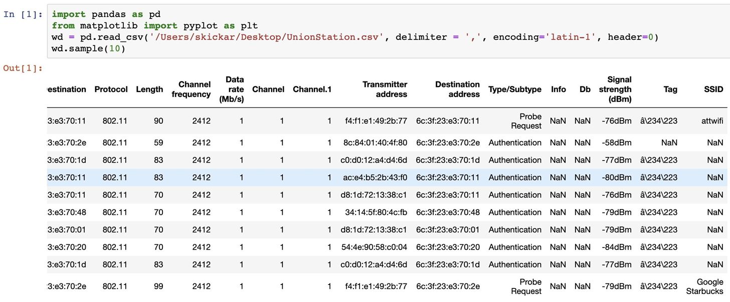
First, we'll import Pandas and nickname it pd, while doing the same with the Pyplot library from Matplotlib as plt. Now, when we refer to pd, Python 3 knows we're talking about Pandas, and the same with plt and Pyplot.

In [ ]: import pandas as pd
        from matplotlib import pyplot as plt

Next, we'll use the Pandas read_csv option to specify the location of the CSV file we're working with, the type of character separating the data (a comma in CSV files or a tab in TSV files), the encoding type, and the row in which the header containing the names of the cells is located. All of this will be put in a variable I named wd or wireless data, but you can call yours whatever you like.

If you're using data like a CSV from Wigle Wifi on an Android phone, it does not use the standard row 0 for headers. You can change the value in this last argument to the row in which the column labels are located to label the data properly.

Finally, we'll sample 10 random data points by using the .sample(10) method to see the results.

In [ ]: wd = pd.read_csv('PATH/TO/FILE.csv', delimiter = ',', encoding='latin-1', header=0)
        wd.sample(10)

Now that we've imported our data, we can start working with it to see what we can learn from the patterns inside it.

Step 4: Plot Basic Data in a Graph

Visualizing data is one of the biggest points of bringing it into Jupyter, so let's dive into exploring relationships with graphs. Go down below the output to a new input, and we'll start slicing through the data.

To do so, we'll need to learn how to access the data inside a data frame. Our complete data frame is our variable, wd, which contains all of the information we imported from our CSV file. To access a piece of the data, we'll use the column names we learned from sampling the data in the last command to access the data in those columns.

If we want to plot the values in the Time column, I can access them using wd[Time].

Knowing that, I can create a graph by first defining the size with the rcParams command, and then plotting the elements I want to graph with the plt.plot(wd[A], wd[B]) command, adding 'o' to indicate we want to use dots rather than lines to plot our data. Finally, we can set the color with the last color variable.

In [ ]: plt.rcParams["figure.figsize"] = (20,10)
        plt.plot(wd['Time'], wd['Transmitter address'], 'o', color='DarkGreen')

The last step will be to label our X and Y axis on the graph.

In [ ]: plt.xlabel('Time')
        plt.ylabel('Real Clients Sending Directed Packets To Fake Networks')

Once this is done, we can add plt.show() to plot the figure.

In [ ]: plt.show()

Now, do the same to plot the "Destination address" column against time as well. The finished result should look something like this.

In [ ]: ## Plotting directed packets (unmasked clients) connecting to fake networks over time
        # Here, we analyze when a clients is connecting to a fake network over time in the first figure.
        # In the second, we analyze which fake networks are recieving directed packets from unmasked clients over time.
        plt.rcParams["figure.figsize"] = (20,10)
        plt.plot(wd['Time'], wd['Transmitter address'], 'o', color='DarkGreen')
        plt.title('Clients Connecting to Fake Networks Over Time')
        plt.xlabel('Time')
        plt.ylabel('Real Clients Sending Directed Packets To Fake Networks')
        plt.show()
        plt.plot(wd['Time'], wd['Destination address'], 'o', color='DarkBlue')
        plt.title('Fake Networks Broadcasted by the Beacon Spammer Recieving Directed Packets')
        plt.xlabel('Time')
        plt.ylabel('Beacon Spammer MAC of Fake Networks Recieving Hit')
        plt.show()

Click on "Run" while you have this input selected to see the result.

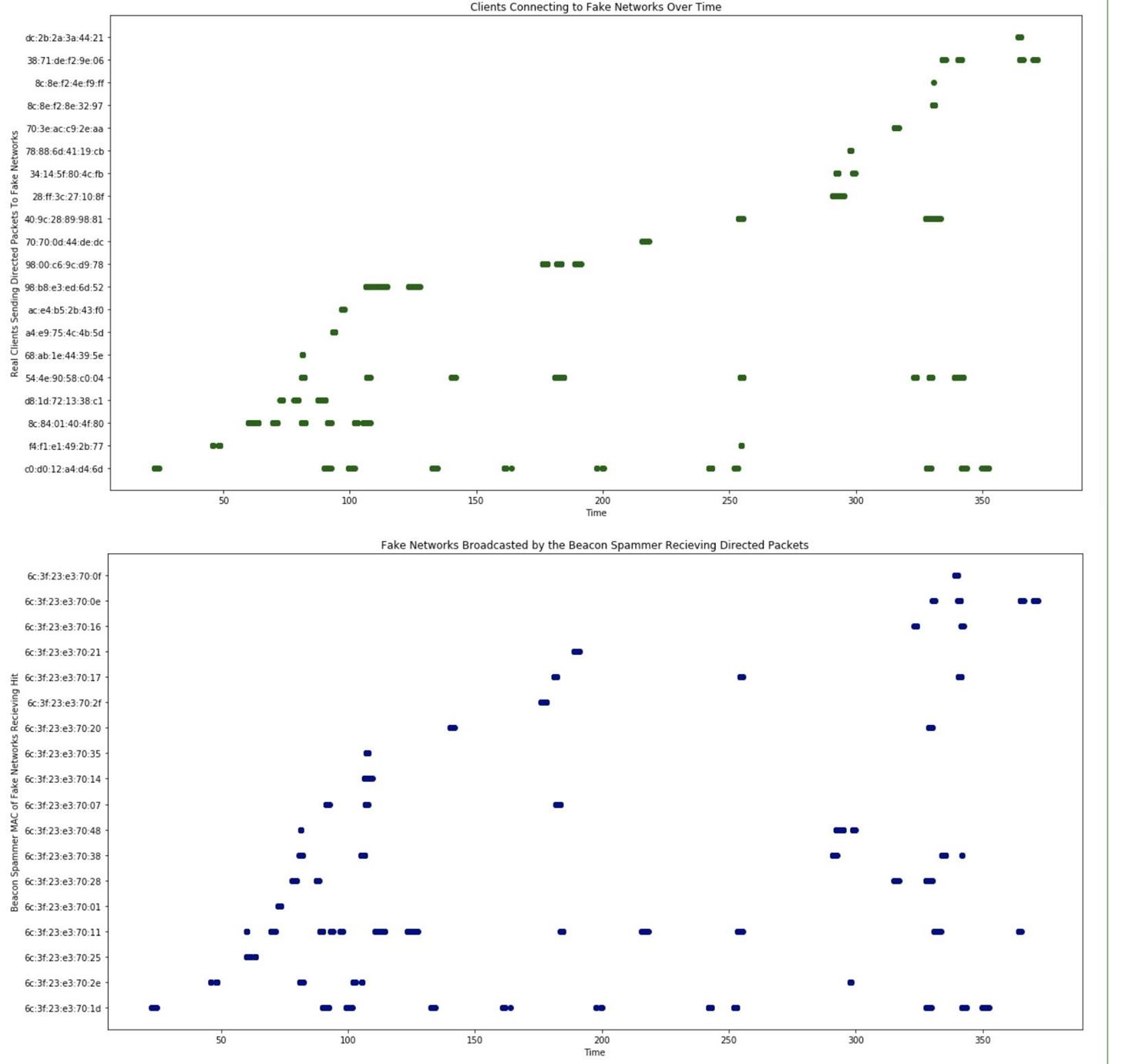
Now, we can see when each real device was transmitting a packet, and when each fake network was receiving a packet. Pretty cool, but let's start looking at fingerprinting engaging networks and clients.

Step 5: Plot Destination & Transmitter Against Each Other

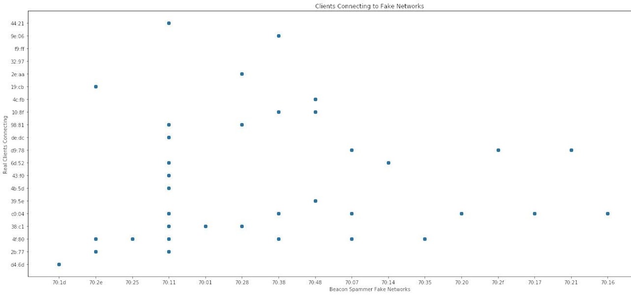
Now, we are going to plot the "Destination address" and "Transmitter address" columns against each other. Doing so will show which networks each device reacted to and which network caused the most devices to react.

To prevent things from getting too long in the labels of the graph, we'll use the .str method to only grab the last five characters of the MAC address in the transmitter and destination field. It should be unique enough for our dataset. To access the last five, we can use an index of -5 and then a : to indicate we want to go to the end of the string. If we wanted the opposite, we could specify :5 to grab the first five. When we call wd[Destination address].str-5:, we're specifying the last five characters in the "Destination address" columns.

After labeling the X and Y axis, the code should look like this:

In [ ]: ## Plotting which client MAC addresses responds to which fake network MAC addresses
        ## Here, we see a fingerprint for every client device on the left.
        ## We can scan the row a device is in to determine which unique fake networks it will respond to.
        ## We can scan a column to find which fake networks cause the most client devices to respond.
        plt.rcParams["figure.figsize"] = (25,10)
        plt.plot(wd['Destination address'].str[-5:], wd['Transmitter address'].str[-5:], 'o',)
        plt.title('Clients Connecting to Fake Networks')
        plt.xlabel('Beacon Spammer Fake Networks')
        plt.ylabel('Real Clients Connecting')
        plt.show()

Click on "Run" to see the results.

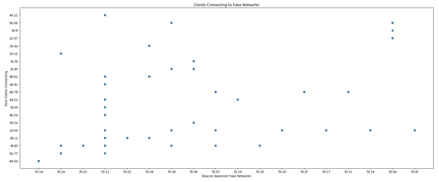
Wow! We can see that each phone seems to have a unique fingerprint. We can also see that one network, in particular, was a lot more popular than the others. That means a hacker could use the network to cause a lot of phones to connect.

Step 6: Find the Most Popular Fake Network

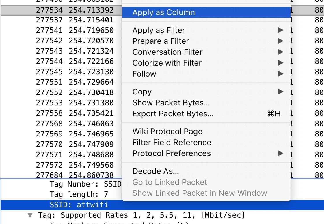
To track down the most popular fake network name nearby devices reacted to, we'll use the same approach of matching the last five characters of the MAC address. In our dataset, there are two types of packets, probe requests and authentication. Probe requests contain the SSID of the network, while authentication does not.

We've captured a lot more authentications than probe requests, so to find out the name of the network all these devices were reacting to, we can search for probe requests with a destination MAC address that matches our popular network's last five characters of "70:11".

We'll do this by using the .str.contains() method, which we can use both for matching the 70:11 string and the Probe frame string. For example, the commandwd[wd['Destination address'].str.contains('70:11') will check if the Destination address field contains the string we're looking for in the MAC address.

Put together, we'll use a variable called popular in which we add any rows that have both a destination address matching that of our mystery network and the word Probe indicating it's a probe request. That should make a list of just probe requests directed at the fake network in question in the popular variable.

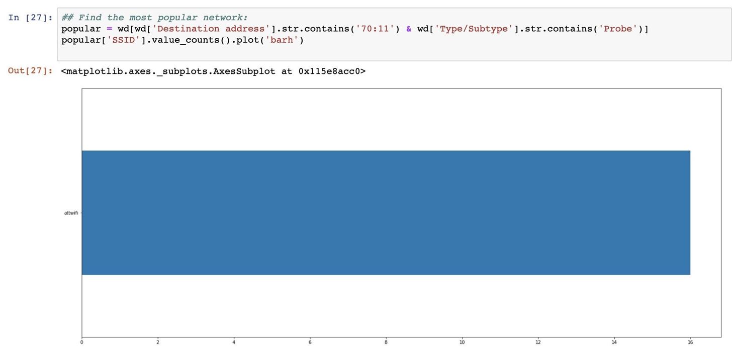
In [ ]: ## Find the most popular network:
        popular = wd[wd['Destination address'].str.contains('70:11') & wd['Type/Subtype'].str.contains('Probe')]

Once we have this list of probe requests, we can graph the data in the "SSID" cell contained with the following command.

In [ ]: popular['SSID'].value_counts().plot('barh')

There we go! Through our analysis, we've determined that the SSID "attwifi" will cause the most number of nearby devices to automatically connect to our fake network.

If we want to share these results with anyone else, we can click the export option to download our notebook in a variety of different formats, including PDF, markdown, and Jupyter's native .ipynb format, which is rendered perfectly on GitHub.

Jupyter Notebook Makes It Easy to Analyze Wi-Fi

Jupyter Notebook hits the sweet spot for analyzing Wi-Fi information, allowing for easy manipulation of massive datasets with simple Python commands. With a little more effort, it's possible to import entire PCAP files raw, but using capture filters and columns in Wireshark to export data in CSV format is a lot more beginner-friendly. I learned Jupyter Notebook in a single evening with only a little bit of Python experience, so I encourage anyone looking for patterns in CSV files to check out this free and easy to use resource.

I hope you enjoyed this guide to deriving insights from Jupyter Notebook and Wireshark! If you have any questions about this tutorial, leave a comment below, and feel free to reach me on Twitter @KodyKinzie.